1 Introduction to Decision Science

1.1 Decision Science

Decision Science is an interdisciplinary field that utilizes advanced analytical methods and tools to facilitate decision-making processes in businesses and organizations.
It combines insights from statistics, economics, psychology, and operational research to analyze and solve problems, enabling leaders to make informed, data-driven decisions.
This essay explores the core concepts of Decision Science, its methodologies, and real-time examples of its application across various industries.

Understanding Decision Science

At its core, Decision Science focuses on the process of making decisions, particularly under conditions of uncertainty.

It involves the study and application of quantitative techniques to analyze complex decision-making scenarios.
The goal is to provide actionable insights that can guide strategic planning, risk management, and problem-solving efforts.

Key Components of Decision Science

Decision science is a multidisciplinary field that utilizes quantitative and qualitative methods for effective decision-making. It draws from various disciplines such as psychology, economics, statistics, and operational research. Below are the key components of decision science:

Data Gathering and Management

This involves the collection, management, and quality assurance of data from diverse sources for analysis.

Statistical Analysis and Modeling

Applies statistical methods and machine learning algorithms to analyze data, identify patterns, and predict outcomes.

Optimization Techniques

Utilizes mathematical models for finding the best possible solutions to problems within certain constraints, including linear and integer programming.

Risk Analysis and Management

Assesses and develops strategies to manage potential risks, understanding the likelihood and impact of different outcomes.

Decision Theory

Studies the principles guiding decision-making, including the evaluation of choices and their outcomes, focusing on concepts like utility and risk preference.

Behavioral Insights

Incorporates psychology and behavioral economics to understand human decision-making, including biases and heuristics.

Prescriptive Analytics

Uses data analysis and modeling to recommend actions for achieving desired outcomes, beyond just predicting future events.

Stakeholder Analysis and Engagement

Identifies and understands the needs and influence of stakeholders involved in or affected by decisions.

Ethics and Responsibility

Considers the ethical implications of decisions to ensure fairness, transparency, and accountability in the decision-making process.

Communication and Visualization

Communicates findings and recommendations effectively through data visualization and clear communication.

Technology and Tools

Employs software and tools for data analysis, modeling, simulation, and visualization to support decision processes.

1.1.1 Methodologies in Decision Science

Decision Science integrates a variety of methodologies to analyze data, inform decision-making, and solve complex problems.
Decision Science employs several methodologies, each suited to different types of decision-making scenarios:

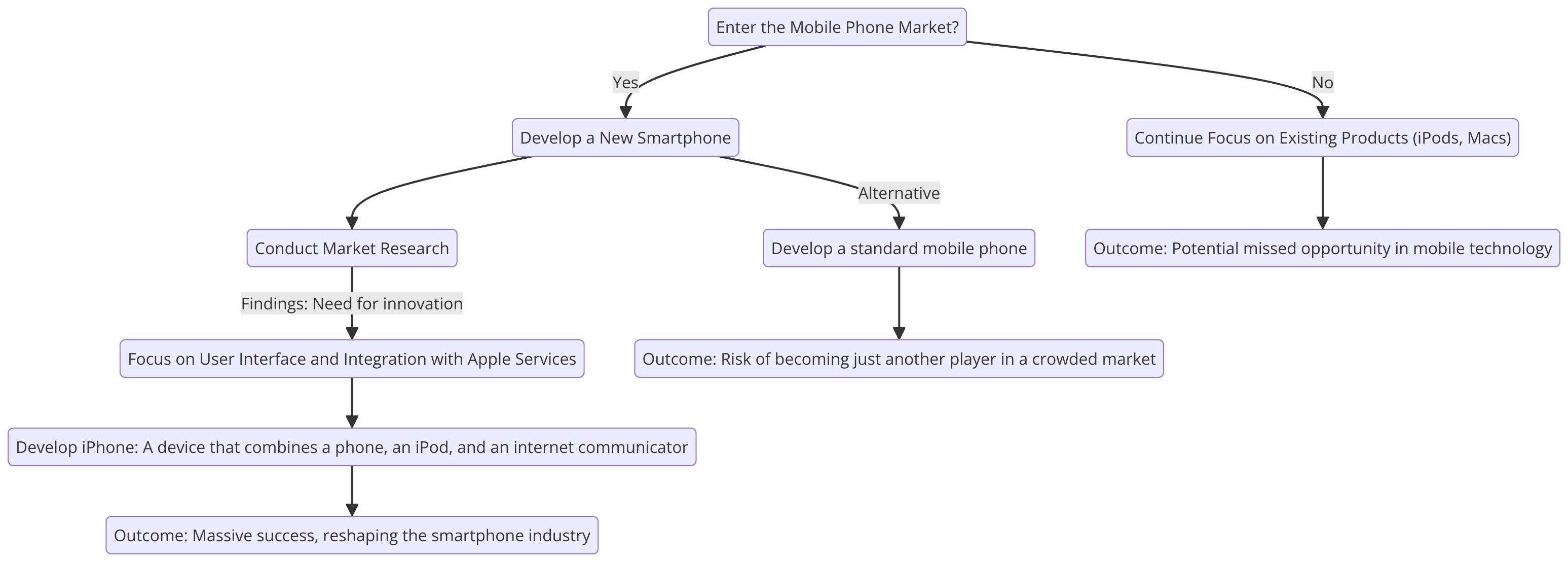
Decision Trees

Visual models that map out various decision paths and their possible outcomes, used for straightforward decisions involving clear, distinct choices.

Apple’s iPhone development decision Tree

Monte Carlo Simulations

A computational technique that uses random sampling to estimate the probabilistic outcomes of a process, useful for decisions under uncertainty.

Linear Programming

A mathematical method for determining the best outcome in a given mathematical model with linear relationships, commonly used for resource allocation problems.

Scenario Analysis

Examines the impact of different scenarios on decision outcomes, helping decision-makers plan for various future states.

1.1.2 Real-Time Examples of Decision Science

Decision Science plays a pivotal role in enhancing operational efficiency, customer satisfaction, and innovation across various sectors. Here, we explore its application in companies like Netflix, Google, Walmart, and Pfizer, highlighting the profound impact on their business.

Netflix

Application

Netflix employs Decision Science to power its content recommendation engine. By analyzing vast amounts of data on user viewing habits, preferences, and interactions, Netflix can recommend personalized content to its subscribers.

Impact

This targeted recommendation system has led to higher viewer engagement rates, reduced churn, and increased subscription renewals. It’s estimated that Netflix’s recommendation engine saves the company over $1 billion annually by minimizing subscription cancellations.

Google

Application

Google applies Decision Science across its product suite, including search algorithms, ad targeting, and new product development. One notable application is in optimizing its data centers’ energy usage through machine learning algorithms.

Impact

By analyzing data on cooling systems and server operations, Google has significantly reduced its data centers’ energy consumption, leading to substantial cost savings and a smaller environmental footprint.

Pfizer

Application

In the pharmaceutical industry, Pfizer uses Decision Science to streamline drug development and improve clinical trial designs. By analyzing historical data and simulations, Pfizer can predict trial outcomes, optimize patient selection, and accelerate the drug development process.

Impact

This approach has led to faster time-to-market for new drugs, reduced development costs, and improved success rates in clinical trials, ultimately benefiting patients with quicker access to new treatments.

Challenges and Future Directions

While Decision Science offers significant benefits, it also faces challenges, including data quality issues, the complexity of modeling real-world scenarios, and the need for interdisciplinary expertise. As technology evolves, Decision Science is increasingly incorporating machine learning and artificial intelligence to enhance decision-making processes. The future of Decision Science lies in its ability to integrate these advanced technologies, offering more sophisticated and automated decision-support systems.

Summary

Decision Science is a vital discipline that empowers organizations to navigate the complexities of the modern business environment. Through the application of rigorous analytical methodologies and the use of real-time data, Decision Science enables informed decision-making that drives strategic success. As the field continues to evolve, its impact on enhancing organizational performance and competitiveness will only grow, marking its significance in the landscape of business and beyond.

1.2 Overview of the Decision-Making Process

Decision Science is a multidisciplinary field that leverages quantitative methods and analytical models to improve decision-making within organizations.
At its heart lies a structured decision-making process that encompasses several stages, from identifying the problem to analyzing outcomes and learning from feedback.

1.2.1 Stages of Decision-Making Process

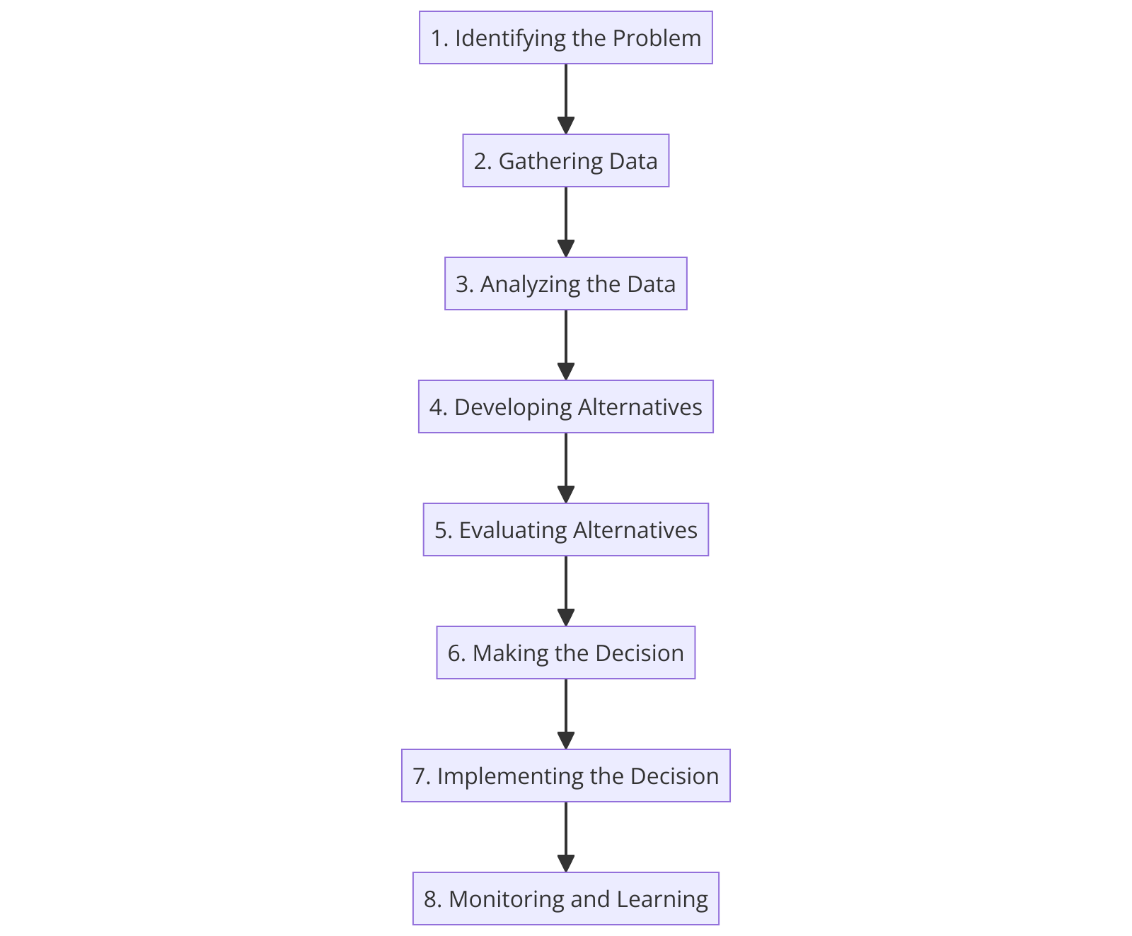
Identifying the Problem

The first step in the decision-making process is recognizing and clearly defining the problem or opportunity. This stage involves understanding the context, stakeholders, and objectives, setting the foundation for targeted analysis and solution development.

Gathering Data

Once the problem is identified, the next step is to collect relevant data. This can involve quantitative data, such as sales figures or operational costs, and qualitative insights, such as customer feedback or employee opinions. Data gathering is crucial for informed analysis and modeling in subsequent stages.

Analyzing the Data

With data in hand, Decision Scientists apply various analytical methods to understand patterns, trends, and relationships. This analysis can range from simple descriptive statistics to complex predictive or prescriptive modeling, depending on the problem’s nature.

Developing Alternatives

Based on the data analysis, multiple solutions or courses of action are developed. This stage requires creativity and strategic thinking to identify viable alternatives that address the problem effectively.

Evaluating Alternatives

Each alternative is then evaluated against a set of criteria, such as cost, feasibility, and impact. Decision Science methodologies, such as decision trees or cost-benefit analysis, can be employed to systematically assess the pros and cons of each option.

Making the Decision

After evaluating the alternatives, the most suitable solution is selected. This decision is based on the comprehensive analysis and alignment with organizational goals and constraints. Decision Science tools can aid in quantifying uncertainty and preferences to make a more informed choice.

Implementing the Decision

The chosen solution is put into action through a detailed implementation plan. This phase involves coordinating resources, communicating with stakeholders, and executing the necessary steps to bring the decision to fruition.

Monitoring and Learning

Finally, the outcomes of the decision are monitored against expectations. This feedback loop is essential for learning, allowing Decision Scientists to refine models, update assumptions, and improve the decision-making process for future challenges.

Summary

The decision-making process in Decision Science is a systematic approach that integrates data analysis, modeling, and strategic thinking to solve complex problems. By following these stages, organizations can make more informed, effective decisions that drive success in an increasingly data-driven world.

Tesla Decision Making Process

Tesla’s strategic decision to champion electric vehicle (EV) technology showcases a comprehensive decision-making process.

Identifying the Problem

Objective: Recognize the environmental drawbacks of fossil fuels and the latent potential in the EV sector.

Gathering Data

Research Areas: Technological advancements in batteries, consumer interest in eco-friendly products, and favorable regulatory developments.

Analyzing the Data

Findings: A significant opportunity exists for luxury EVs offering both performance and sustainability.

Developing Alternatives

Options Considered: Focus on hybrid models, license existing technology, or develop a full EV lineup.

Evaluating Alternatives

Criteria: Environmental impact, market uniqueness, and potential for long-term success.

Making the Decision

Resolution: Commit to manufacturing high-end, fully electric vehicles, starting with the Roadster to finance subsequent mass-market models.

Implementing the Decision

Execution: Launch the Tesla Roadster, followed by the Model S, Model X, and the more accessible Model 3.

Monitoring and Learning

Adjustments: Ongoing innovation in battery technology, software, and manufacturing, informed by market response and tech progress.

1.3 Rationality and Decision Theory

Rationality and decision theory are central to understanding decision-making in economics, psychology, and philosophy. These concepts help explain how individuals and organizations choose among available options to maximize their outcomes.

1.3.1 Rationality in Decision Making

Rationality involves making decisions based on logical reasoning and factual evidence, aiming to maximize utility or satisfaction. It encompasses a systematic process of identifying goals, evaluating alternatives, and selecting the most beneficial option.

Types of Rationality

Instrumental Rationality: This type involves choosing the most effective means to achieve a given end, assuming the end is rational.
Epistemic Rationality: This pertains to beliefs and their adjustment based on evidence and logical reasoning, focusing on forming and updating beliefs accurately.

1.3.2 Decision Theory: Normative and Descriptive Approaches

Decision theory splits into two branches, each offering a different perspective on decision-making processes:

Normative Decision Theory (Prescriptive): This branch uses mathematical models to prescribe optimal decision-making strategies, focusing on how decisions should be made.
Descriptive Decision Theory: This branch examines actual decision-making behaviors, including biases and irrationalities, to understand and predict human actions.

1.3.3 Challenges to Rationality

Despite the ideal of making rational decisions, several factors complicate this process in practice:

Limited Information: Decision-makers often lack complete information, making it difficult to consider all possible outcomes.
Cognitive Biases: Psychological biases can lead to irrational decision-making that deviates from optimal choices.
Bounded Rationality: A concept introduced by Herbert A. Simon, suggesting that individuals make rational decisions within the limits of their information and cognitive capabilities.

1.3.4 Real-World Application

Business Strategy

Companies use tools like decision trees and cost-benefit analyses for strategic planning and investment decisions, aiming to optimize outcomes based on available data and objectives.

Public Policy

Rational choice theory is applied in public policy to design regulations and policies that influence or control behavior in predictable ways.

Summary

Understanding rationality and decision theory is essential for making informed, optimal decisions in various fields. While challenges exist, including limited information and cognitive biases, these concepts provide a valuable framework for analyzing and improving decision-making processes.

1.4 Types of Decisions

1. Strategic Decisions

Strategic decisions set the direction for the entire organization and have long-term implications. These decisions are typically made at the highest levels of management and involve significant investment and risk.

Example: A tech company deciding to acquire a smaller startup to enter the virtual reality market. This strategic move is aimed at positioning the company in a fast-growing segment, requiring thorough market analysis, financial forecasting, and consideration of the cultural integration of the two companies.

2. Tactical Decisions

Tactical decisions are concerned with the implementation of strategic decisions. They are medium-term, more specific, and involve managing resources efficiently to achieve strategic objectives.

Example: A retail chain deciding to implement a new inventory management system to optimize stock levels and reduce holding costs. This involves selecting the right software, training employees, and integrating the system with the supply chain.

3. Operational Decisions

Operational decisions are routine decisions that support the day-to-day operations of an organization. These are often short-term and involve specific tasks and processes.

Example: A restaurant manager creating a weekly work schedule to ensure that staffing meets the anticipated customer demand, taking into account employees’ availability and peak dining times.

4. Programmed Decisions

Programmed decisions are routine decisions that follow a standard procedure or rule. These are typically automated or require minimal judgment.

Example: A bank uses an automated system to approve or reject loan applications based on predefined criteria such as credit score, income, and employment history.

5. Non-Programmed Decisions

Non-programmed decisions occur in response to unusual or novel situations that have not been encountered before. These decisions require creativity, judgment, and a tailored approach.

Example: A company’s executive team devising a strategy to respond to a new, disruptive technology introduced by a competitor, affecting their market share and requiring a unique, innovative response.

1.4.1 Nature of Decision Problems

1. Structured Problems

Structured problems are clear, well-defined, and often quantitative, allowing for straightforward solutions using standard procedures

Example: Determining the reorder point for a high-demand product using historical sales data and inventory levels.

2. Unstructured Problems

Unstructured problems are complex, ambiguous, and involve high levels of uncertainty. They require significant analysis, judgment, and creative problem-solving

Example: Developing a strategy to enter an emerging market with a new product, where market dynamics, customer preferences, and competitive landscape are largely unknown.

3. Semi-Structured Problems

Semi-structured problems contain elements of both structured and unstructured problems. They require a combination of analytical approaches and judgment-based decision-making.

Example: Deciding on the marketing mix for a new product launch, where some elements like the target audience and product features are known, but the optimal pricing and promotional channels need to be determined through analysis and experimentation.

4. Decision Making under Certainty

Decisions made under certainty involve situations where all necessary information is known, and the outcome of each decision option is predictable.

Example: Calculating the production schedule for a manufacturing plant when demand for the next month is known and stable.

5. Decision Making under Uncertainty

Decisions under uncertainty are made when the decision-maker lacks complete information, and it is not possible to determine the likelihood of various outcomes

Example: A pharmaceutical company deciding whether to invest in the research and development of a new drug without knowing whether it will be successful or approved by regulatory bodies.

6. Decision Making under Risk

Decision-making under risk involves situations where the outcomes are uncertain, but the probability of each outcome can be estimated, allowing for informed decision-making.

Example: An investment firm allocating assets in its portfolio, using historical data and statistical models to estimate the risk and return of various investment options.

1.5 Decision Trees and Probability Theory

Presentation

1.5.1 Decision Tree

A decision tree is one of the most powerful tools of supervised learning algorithms used for both classification and regression tasks.
It builds a flowchart-like tree structure where each internal node denotes a test on an attribute, each branch represents an outcome of the test, and each leaf node (terminal node) holds a class label.
It is constructed by recursively splitting the training data into subsets based on the values of the attributes until a stopping criterion is met, such as the maximum depth of the tree or the minimum number of samples required to split a node.
During training, the Decision Tree algorithm selects the best attribute to split the data based on a metric such as entropy or Gini impurity, which measures the level of impurity or randomness in the subsets.
The goal is to find the attribute that maximizes the information gain or the reduction in impurity after the split.

Decision Tree Terminologies

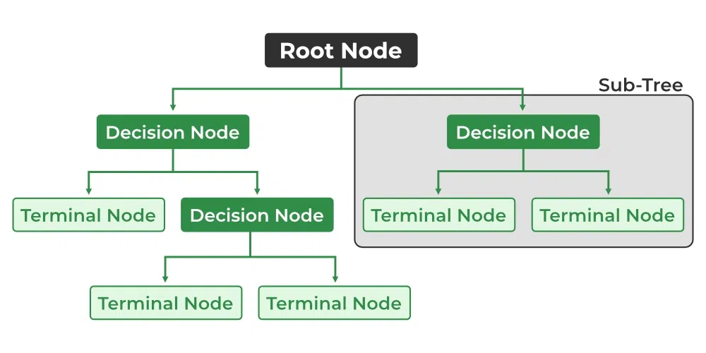
Root Node

It is the topmost node in the tree, which represents the complete dataset. It is the starting point of the decision-making process.

Decision/Internal Node

A node that symbolizes a choice regarding an input feature. Branching off of internal nodes connects them to leaf nodes or other internal nodes.

Leaf/Terminal Node

A node without any child nodes that indicates a class label or a numerical value.

Splitting

The process of splitting a node into two or more sub-nodes using a split criterion and a selected feature.

Branch/Sub-Tree

A subsection of the decision tree starts at an internal node and ends at the leaf nodes.

Parent Node

The node that divides into one or more child nodes.

Child Node

The nodes that emerge when a parent node is split.

Impurity

A measurement of the target variable’s homogeneity in a subset of data. It refers to the degree of randomness or uncertainty in a set of examples. The Gini index and entropy are two commonly used impurity measurements in decision trees for classification tasks.

Variance

Variance measures how much the predicted and the target variables vary in different samples of a dataset. It is used for regression problems in decision trees. Mean squared error, Mean Absolute Error, friedman_mse, or Half Poisson deviance are used to measure the variance for the regression tasks in the decision tree.

Information Gain

Information gain is a measure of the reduction in impurity achieved by splitting a dataset on a particular feature in a decision tree. The splitting criterion is determined by the feature that offers the greatest information gain. It is used to determine the most informative feature to split on at each node of the tree, with the goal of creating pure subsets.

Gini Impurity is a score that evaluates how accurate a split is among the classified groups. The Gini Impurity evaluates a score in the range between 0 and 1, where 0 is when all observations belong to one class, and 1 is a random distribution of the elements within classes.
In this case, we want to have a Gini index score as low as possible. Gini Index is the evaluation metric we shall use to evaluate our Decision Tree Model.

Pruning

The process of removing branches from the tree that do not provide any additional information or lead to overfitting.

This terminology forms the foundation of decision tree models, helping to elucidate the process from dataset analysis to the formulation of decision rules based on the features within the data.

Entropy

Entropy is the measure of the degree of randomness or uncertainty in the dataset. In the case of classifications, It measures the randomness based on the distribution of class labels in the dataset.

Important points related to Entropy:

The entropy is 0 when the dataset is completely homogeneous, meaning that each instance belongs to the same class. It is the lowest entropy indicating no uncertainty in the dataset sample.
When the dataset is equally divided between multiple classes, the entropy is at its maximum value. Therefore, entropy is highest when the distribution of class labels is even, indicating maximum uncertainty in the dataset sample.
Entropy is used to evaluate the quality of a split. The goal of entropy is to select the attribute that minimizes the entropy of the resulting subsets, by splitting the dataset into more homogeneous subsets with respect to the class labels.
The highest information gain attribute is chosen as the splitting criterion (i.e., the reduction in entropy after splitting on that attribute), and the process is repeated recursively to build the decision tree.

1.5.2 Decision Tree Assumptions

Several assumptions are made to build effective models when creating decision trees. These assumptions help guide the tree’s construction and impact its performance. Here are some common assumptions and considerations when creating decision trees:

Binary Splits

Decision trees typically make binary splits, meaning each node divides the data into two subsets based on a single feature or condition. This assumes that each decision can be represented as a binary choice.

Recursive Partitioning

Decision trees use a recursive partitioning process, where each node is divided into child nodes, and this process continues until a stopping criterion is met. This assumes that data can be effectively subdivided into smaller, more manageable subsets.

Feature Independence

Decision trees often assume that the features used for splitting nodes are independent. In practice, feature independence may not hold, but decision trees can still perform well if features are correlated.

Homogeneity

Decision trees aim to create homogeneous subgroups in each node, meaning that the samples within a node are as similar as possible regarding the target variable. This assumption helps in achieving clear decision boundaries.

Top-Down Greedy Approach

Decision trees are constructed using a top-down, greedy approach, where each split is chosen to maximize information gain or minimize impurity at the current node. This may not always result in the globally optimal tree.

Categorical and Numerical Features

Decision trees can handle both categorical and numerical features. However, they may require different splitting strategies for each type.

Overfitting

Decision trees are prone to overfitting when they capture noise in the data. Pruning and setting appropriate stopping criteria are used to address this assumption.

Impurity Measures

Decision trees use impurity measures such as Gini impurity or entropy to evaluate how well a split separates classes. The choice of impurity measure can impact tree construction.

No Missing Values

Decision trees assume that there are no missing values in the dataset or that missing values have been appropriately handled through imputation or other methods.

Equal Importance of Features

Decision trees may assume equal importance for all features unless feature scaling or weighting is applied to emphasize certain features.

No Outliers

Decision trees are sensitive to outliers, and extreme values can influence their construction. Preprocessing or robust methods may be needed to handle outliers effectively.

Sensitivity to Sample Size

Small datasets may lead to overfitting, and large datasets may result in overly complex trees. The sample size and tree depth should be balanced.

1.5.3 Probability Theory

Probability theory is a branch of mathematics concerned with analyzing random phenomena. It provides a framework for quantifying the likelihood of events, ranging from everyday occurrences to sophisticated scientific experiments. The fundamental concept of probability theory is the “probability,” a measure that assigns a number between 0 and 1 to indicate how likely an event is to occur, with 0 representing impossibility and 1 certainty.

Basic Concepts

Random Experiment

In probability theory, any event which can be repeated multiple times and its outcome is not hampered by its repetition is called a Random Experiment. Tossing a coin, rolling dice, etc. are random experiments.

Sample Space

The set of all possible outcomes for any random experiment is called sample space. For example, throwing dice results in six outcomes, which are 1, 2, 3, 4, 5, and 6. Thus, its sample space is (1, 2, 3, 4, 5, 6)

Event

The outcome of any experiment is called an event. Various types of events used in probability theory are,

Independent Events: The events whose outcomes are not affected by the outcomes of other future and/or past events are called independent events. For example, the output of tossing a coin in repetition is not affected by its previous outcome.
Dependent Events: The events whose outcomes are affected by the outcome of other events are called dependent events. For example, picking oranges from a bag that contains 100 oranges without replacement.
Mutually Exclusive Events: The events that can not occur simultaneously are called mutually exclusive events. For example, obtaining a head or a tail in tossing a coin, because both (head and tail) can not be obtained together.
Equally likely Events: The events that have an equal chance or probability of happening are known as equally likely events. For example, observing any face in rolling dice has an equal probability of 1/6.
Probability of an Event (P(E)): A measure of the likelihood that the event will occur. It is calculated as the number of favorable outcomes to the event divided by the total number of possible outcomes in the sample space.

Types of Probability

Classical Probability: Assumes that all outcomes in the sample space are equally likely. It is calculated as the ratio of the number of favorable outcomes to the total number of outcomes.
Empirical Probability: Based on observations or experiments. It is calculated as the ratio of the number of times an event occurs to the total number of trials or observations.
Subjective Probability: Based on belief or experience, without any objective calculation. It varies from person to person.

Key Principles

The Law of Large Numbers: States that as more observations are collected, the actual ratio of outcomes will converge on the theoretical, or expected, ratio of outcomes.
The Addition Rule: Provides a way to calculate the probability of either of two events happening.
The Multiplication Rule: Allows the calculation of the probability that two events will happen together.

Probability Distributions

Probability distributions describe how probabilities are distributed over the values of the random variable. They can be classified into discrete and continuous distributions.

Discrete Probability Distributions: Concerned with outcomes that can be counted. Examples include the binomial and Poisson distributions.
Continuous Probability Distributions: Deal with outcomes that can take any value within a range. Examples include the normal (Gaussian) and uniform distributions.

Applications

Probability theory is fundamental in various fields such as finance, insurance, science, engineering, and everyday decision-making. It forms the basis for statistical inference, enabling the analysis and interpretation of data, hypothesis testing, and prediction.

Probability theory provides a vital foundation for understanding uncertainty and making informed decisions under conditions of uncertainty. Its principles and methodologies enable us to quantify the likelihood of events, assess risks, and predict future outcomes, making it an indispensable tool in a wide array of disciplines.

Essential formulas

To complement the explanation of probability theory, here are some essential formulas that are foundational to understanding and working with probabilities:

Basic Probability Formula

The probability of an event $A$ occurring in a finite sample space is given by: \[ P(A) = \frac{\text{Number of favorable outcomes to } A}{\text{Total number of possible outcomes in the sample space}} \]

The Addition Rule

For any two events $A$ and $B$, the probability that $A$ or $B$ occurs is: \[ P(A \cup B) = P(A) + P(B) - P(A \cap B) \] If $A$ and $B$ are mutually exclusive (cannot happen at the same time), then: \[ P(A \cup B) = P(A) + P(B) \]

The Multiplication Rule

For any two events $A$ and $B$, the probability that both $A$ and $B$ occur is: \[ P(A \cap B) = P(A) \times P(B|A) \] If $A$ and $B$ are independent (the occurrence of one does not affect the occurrence of the other), then: \[ P(A \cap B) = P(A) \times P(B) \]

Conditional Probability

The probability of $A$ given $B$ has occurred is: \[ P(A|B) = \frac{P(A \cap B)}{P(B)} \]

Bayes’ Theorem

Bayes’ Theorem provides a way to update our probability estimates on new evidence: \[ P(A|B) = \frac{P(B|A) \times P(A)}{P(B)} \]

Expected Value

For a discrete random variable $X$ with possible values $x_1, x_2, \ldots, x_n$ and probabilities $P(x_1), P(x_2), \ldots, P(x_n)$, the expected value ($E[X]$) is: \[ E[X] = \sum_{i=1}^{n} x_i P(x_i) \]

For a continuous random variable $X$ with probability density function $f(x)$, the expected value is: \[ E[X] = \int_{-\infty}^{\infty} x f(x) dx \]

Variance

The variance of a random variable $X$ measures the spread of its values and is defined as: \[ \text{Var}(X) = E[(X - E[X])^2] = E[X^2] - (E[X])^2 \]

These formulas are crucial for performing probability calculations, making predictions, and conducting statistical analyses. Understanding and applying these concepts allows us to navigate uncertainty and make informed decisions in various disciplines.